Fig. 5.26: Schematic of an abstract LAN Ethernet network
The workstation model in AleC++ is as follows.
While the previous example shows Alecsis use in gate-level logic simulation, this one will illustrate its capabilities at higher levels of abstraction. Using signals typed as classes, it is possible to create complex inter-process communication. Fig. 5.26 shows Local Area Network (LAN) modeled using AleC++ discrete-event simulation constructs. Each workstation is represented as an autonomous concurrent process with its own activity pattern. LAN cable segments between stations are modeled as simple bi-directional buffers that pass information with some transport delay proportional to the cable length. After non-deterministic idle periods calculated using the uniform random distribution, the stations attempt to send their frames, according to CSMA/CD protocols [Watk93, Schw87]. After sending the frame, the station monitors the line for the specified period (2*slot_size), and then compare the original and the frame on the line. If they are not the same, the collision took place, and the frames are scheduled for retransmission after a period calculated using binary exponential backoff algorithm. According to CD (Collision Detection) strategy, the station is capable of truncating the corrupted frame without waiting 2*slot_size period in case of collision.
Fig. 5.26: Schematic of an abstract LAN Ethernet network
The workstation model in AleC++ is as follows.
enum StationState { NormalState, CollisionState };
module LAN::workstation(frame inout lan_port) {
}action (int id, const char *ws_name) {
process {
frame last_frame;
double last_sent = 0.0;
StationState ss = NormalState;
int ntrials = 0;if (ss == NormalState) {
wait for idle_period();
last_sent = now;if ( !lan_port.status (FreeLine) )
wait lan_port while
!lan_port.status(FreeLine);}
last_frame.stamp(NormalFrame, id, receiver(id, nst), now, ws_name);
lan_port <- last_frame;
last_sent = now;
wait lan_port for listen_period();if ( last_frame != lan_port ) {
if (ss == NormalState) {
ntrials = 0;
ss = CollisionState;}
ntrials++;
if(ntrials > max_trials() ) {ss = NormalState; // discard frame
ntrials = 0;} else {
lan_port <- frame(NoiseBurst, now);
wait for burst_period();
lan_port <- frame(FreeLine, now);
wait for retrans_period(ntrials);}
} else { // successful transmission
ss = NormalState;
lan_port <- frame(NoiseBurst, now);
wait for burst_period();
lan_port <- frame(FreeLine, now);
last_frame.stamp(FreeLine,0,0,now,ws_name);}
}
}
The complete modeling procedure for this problem is explained in [Maks95].
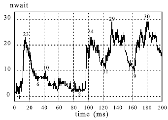
As in all previous examples, workstation modules are parametrized using model card class. That gives an opportunity to create model cards of real workstations, with different idle times and activity patterns. Fig. 5.27 shows the simulation results of an abstract LAN Ethernet network with 50 workstations interconnected with 5m cable segments. The stations were idle from 0 to 10ms, while the simulation covered 0.2s time period. The curve represents number of stations waiting to transmit their frames due to the occupied line. All the stations were capable of gathering the statistical data about network performance. Post processing of those data carried out in a process synchronized using implicit signal final showed that 712 frames were sent successfully, while 1319 frames were re-transmitted due to a collision. The total transmission delay was 2.43s, average delay per station 47.6ms, and average delay per frame 3.47ms.
Fig. 5.27: Simulation results of the LAN Ethernet network with 50 workstations. The curve represents number of stations waiting to transmit their frames due to occupied line.
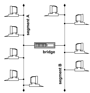
As the next example, the Ethernet bridge modeling and simulation will be considered.
The Ethernet bridge, as shown in Fig. 5.28, interconnects network segments. The network layer as well as all other (transport, session, presentation and application) layers are not affected by the bridge, so that the bridge is totally transparent to the user. Two main functions of the bridge are: filtering traffic (bridges provide for a filtering component to improve network performance) and bridging media. (Bridges frequently interconnect different networks. These networks are often Ethernet or token ring. The bridges merely duplicate all signals originating from all source networks and send them to other networks.)
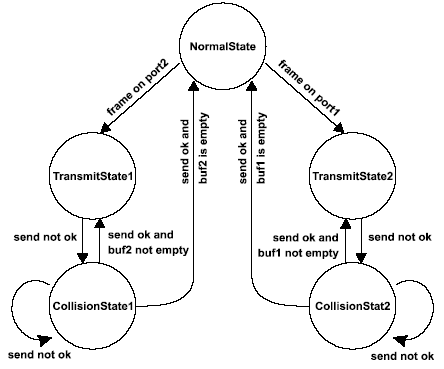
In the example considered here, the bridge has two LAN-boards because it interconnects two segments. The received frame on one board ( port1 ) has to be transferred by the bridge to another segment via appropriate LAN-board ( port2 ). In operation mode, the bridge may be in one of the following five states:
1. NormalState - in this state the bridge waits to receive frames
2. TransmisionState1 - in this state bridge attempts to send a frame to port 1
3. CollisionState1 - in this state, after collision, the bridge resends the frame to port 1
4. TransmisionState2 - in this state the bridge attempts to send a frame to port 2
5. CollisionState2 - in this state, after collision, the bridge resends the frame to port 2.
Fig. 5.28: Ethernet LAN with a bridge
The state-transition diagram used for modeling is presented in Fig. 5.29 in a form of an oriented graph. For simulation purposes, in addition to the network topology and functionality, the time properties for every network element and delay times for every state transition should be given. The next AleC++ code describes a bridge in a computer network.
Fig. 5.29: State-transition diagram used for bridge modeling
//libr. lanb contains modules: cable,workstation,bridge,... library lanb;
// model cards for stations and bridge
model LAN::sgi_indigo {
frame_size=256; max_retrans=16; idle_time=IdleTime;
} model LAN::hp9000 {
frame_size=256; max_retrans=16; idle_time=IdleTime;
} model LAN::bridge2 { frame_size=256; max_retrans=16; }
...
root module net_with_bridge ( ) {
// declarations of workstations, cables and bridge
module workstation w1, w2, ... ;
cable c_1, c_2, ... ;
module bridge b1;
...
// signal declarations signal cable_t w1_port={FreeLine}, w2_port={FreeLine};
signal cable_t b1_port1={FreeLine}, b1_port2={FreeLine};
signal cable_t term_1={FreeLine}, term_2={FreeLine};
...
// instantiation
w1(w1_port) {
ws_name="indigo";
id=5;
nst=numst;
model=sgi_indigo;}
w2(w2_port) {
ws_name="hp";
d=6;
nst=numst;
model=hp9000;}
b1 (b1_port1, b1_port2) {
bg_name="bg301";
id=20;
model=bridge2;}
c_5 (w1_port, w2_port) cable_delay = Ldelay(4.0_meter);
c_2 (w1_port, b1_port1) cable_delay = Ldelay(5.0_meter);
c_6 (w2_port, term_2) cable_delay = Ldelay(0.1_meter);
...
timing { tstop = 13*IdleTime; }
...
}
As simulation result, statistics are obtained related to all the stations, the bridge (see Table 5.3), and overall network. Table 5.3 contains two kinds of data: number of frames is given in the first five rows, while the last two rows represent delays caused by the data transfer through the bridge.
Table 5.3: Bridge activity statistics
|
Bridge |
Port 1 |
Port 2 |
received frames total |
60 |
43 |
17 |
for transmission |
25 |
18 |
7 |
successful |
23 |
16 |
7 |
unsuccessful |
2 |
2 |
0 |
repeated |
14 |
12 |
2 |
total delay [s] |
0.0062464 |
|
|
mean delay [s/frame] |
0.0001041 |
|
|